Chapter 13 Adjustments and comparisons
It’s fairly common to make adjustments to the index, perhaps in terms of alternative data sets, indicators, methodological decisions, and so on. COINr allows you to (a) make fast adjustments, and (b) to compare alternative versions of the index relatively easily.
13.1 Regeneration
One of the key advantages of working within the “COINrverse” is that (nearly) all the methodology that is applied when building a composite indicator (COIN) is stored automatically in a folder of the COIN called .$Method. To see what this looks like:
# load COINr if not loaded
library(COINr6)

# build example COIN
ASEM <- build_ASEM()
## -----------------
## Denominators detected - stored in .$Input$Denominators
## -----------------
## -----------------
## Indicator codes cross-checked and OK.
## -----------------
## Number of indicators = 49
## Number of units = 51
## Number of aggregation levels = 3 above indicator level.
## -----------------
## Aggregation level 1 with 8 aggregate groups: Physical, ConEcFin, Political, Instit, P2P, Environ, Social, SusEcFin
## Cross-check between metadata and framework = OK.
## Aggregation level 2 with 2 aggregate groups: Conn, Sust
## Cross-check between metadata and framework = OK.
## Aggregation level 3 with 1 aggregate groups: Index
## Cross-check between metadata and framework = OK.
## -----------------
## Missing data points detected = 65
## Missing data points imputed = 65, using method = indgroup_mean

# look in ASEM$Method folder in R Studio...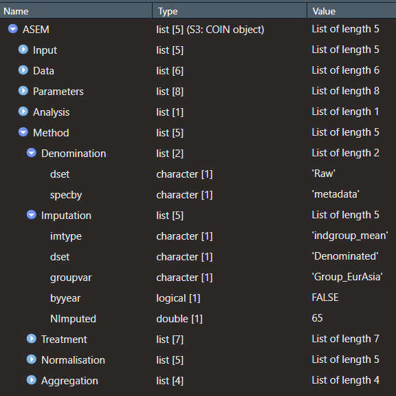
Figure 13.1: Method folder in ASEM example
The easiest way to view it is by looking in the viewer of R Studio as in the screenshot above. Essentially, the .$Method folder has one entry for each COINr function that was used to build the COIN, and inside each of these folders are the arguments to the function that were input. Notice that the names inside .$Method$denominate correspond exactly to arguments to denominate(), for example.
Every time a COINr “construction function” is run, the inputs to the function are automatically recorded inside the COIN. Construction functions are any of the following seven:
| Function | Description |
|---|---|
assemble() |
Assembles indicator data/metadata into a COIN |
checkData() |
Data availability check and unit screening |
denominate() |
Denominate (divide) indicators by other indicators |
impute() |
Impute missing data using various methods |
treat() |
Treat outliers with Winsorisation and transformations |
normalise() |
Normalise data using various methods |
aggregate() |
Aggregate indicators into hierarchical levels, up to index |
These are the core functions that are used to build a composite indicator, from assembling from the original data, up to aggregation.
One reason to do this is simply to have a record of what you did to arrive at the results. However, this is not the main reason (and in fact, it would be anyway good practice to make your own record by creating a script or markdown doc which records the steps). The real advantage is that results can be automatically regenerated with a handy function called regen().
To regenerate the results, simply run e.g.:
ASEM2 <- regen(ASEM)
## -----------------
## Denominators detected - stored in .$Input$Denominators
## -----------------
## -----------------
## Indicator codes cross-checked and OK.
## -----------------
## Number of indicators = 49
## Number of units = 51
## Number of aggregation levels = 3 above indicator level.
## -----------------
## Aggregation level 1 with 8 aggregate groups: Physical, ConEcFin, Political, Instit, P2P, Environ, Social, SusEcFin
## Cross-check between metadata and framework = OK.
## Aggregation level 2 with 2 aggregate groups: Conn, Sust
## Cross-check between metadata and framework = OK.
## Aggregation level 3 with 1 aggregate groups: Index
## Cross-check between metadata and framework = OK.
## -----------------
## Missing data points detected = 65
## Missing data points imputed = 65, using method = indgroup_mean
The regen() function reruns all functions that are recorded in the .$Method folder in the order they appear in the folder. In this example, it runs, in order, assemble(), denominate(), impute(), treat(), normalise()and aggregate(). This replicates exactly the results. But what is the point of that? Well, it means that we can make changes to the index, generally by altering parameters in the .$Method folder, and then rerun everything very quickly with a single command. This will be demonstrated in the following section. After that, we will also see how to compare between alternative versions of the index.
Before that, there is one extra feature of regen() which is worth mentioning. The regen() function only runs the seven construction functions as listed above. These functions are very flexible and should encompass most needs for constructing a composite indicator. But what happens if you want to build in an extra operation, or operations, that are outside of these seven functions?
It is possible to also include “custom” chunks of code inside the COIN. Custom chunks should be written manually using the quote() function, to a special folder .$Method$Custom. These chunks can be any type of code, but the important thing is to also know when to run the code, i.e. at what point in the construction process.
More specifically, custom code chunks are written as a named list. The name of the item in the list specifies when to perform the operation. For example, “after_treat” means to perform this immediately after the treatment step. Other options are e.g. “after_normalise” or “after_impute” – in general it should be “after_” followed by a name of one of the names of the construction functions.
The corresponding value in the list should be an operation which must be enclosed in the quote() function. Clearly, the list can feature multiple operations at different points in construction. The COIN is referred to by the generic name COIN, rather than the name you have assigned to your COIN.
This is slightly complicated, but can be clarified a bit with an example. Let’s imagine that after Winsorisation, we would like to “reset” one of the Winsorised points to its original value. This is currently not possible inside the treat() function so has to be done manually. But we would like this operation to be kept when we regenerate the index with variations in methodology (e.g. trying different aggregation functions, weights, etc.).
We create a list with one operation: resetting the point after the treatment step.
# Create list. NOTE the use of the quote() function!
custlist = list(after_treat = quote(COIN$Data$Treated$Bord[COIN$Data$Treated$UnitCode=="BEL"] <- COIN$Data$Imputed$Bord[COIN$Data$Imputed$UnitCode=="BEL"]))

# Add the list to the $Method$Custom folder
ASEM$Method$Custom <- custlist
Specifically, we have replaced the Winsorised value of Belgium, for the “Bord” indicator, with its imputed value (i.e. the value it had before it was treated).
Now, when we regenerate the COIN using regen(), it will insert this extra line of code immediately after the treatment step. Clearly, anything we refer to in this custom code must be available at that step in the construction. For example, we can’t refer to the aggregated data set if the data has not yet been aggregated.
Using custom code may seem a bit confusing but it adds an extra layer of flexibility. It is however intended for small snippets of custom code, rather than large blocks of custom operations. If you are doing a lot of operations outside COINr, it may be better to do this in your own dedicated script or function, rather than trying to encode absolutely everything inside the COIN. However, also consider that some features of COINr, such as global sensitivity analysis, require everything to be encoded inside the COIN.
Before moving on, it’s worth reiterating that regenerating a COIN runs the construction functions in the order they appear in the Method folder. That means that if you build an index with no imputation, for example, and then later decide to make a copy which now includes imputation, you would have to insert the .Method$imputation entry in the place where it should occur. An easy way to do this is using R’s append() function.
13.2 Adjustments
Let us now explore how the COIN can be adjusted and regenerated. This will (hopefully) clarify why regenerating is a useful thing.
The general steps for adjustments are:
- Copy the object
- Adjust the index methodology or data by editing the
.$Methodfolder and/or the underlying data - Regenerate the results
- Compare alternatives
Copying the object is straightforward, and regeneration has been dealt with in the previous section. Comparison is also addressed in the following section. Here we will focus on adjustments and changing methodology.
13.2.1 Adding/removing indicators
First of all, let’s consider an alternative index where we decide to add or remove one or more indicators. There are different ways that we could consider doing this.
A first possibility would be to manually create a new data frame of indicator data and indicator metadata, i.e. the IndData and IndMeta inputs for assemble(). This is fine, but we would have to start the index again from scratch and rebuild it.
A better idea is that when we first supply the set of indicators to assemble(), we include all indicators that we might possibly want to include in the index, including e.g. alternative indicators with alternative data sources. Then we build different versions of the index using subsets of these indicators. This allows us to use regen() and therefore to make fast copies of the index.
To illustrate, consider again the ASEM example. We can rebuild the ASEM index using a subset of the indicators by using the include or exclude arguments of the assemble() function. Because these are stored in .$Method, we can easily regenerate the new results.
# Make a copy
ASEM_NoLPIShip <- ASEM

# Edit method: exclude two indicators
ASEM_NoLPIShip$Method$assemble$exclude <- c("LPI", "Ship")

# Regenerate results (suppress any messages)
ASEM_NoLPIShip <- regen(ASEM_NoLPIShip, quietly = TRUE)
Note that, in the ASEM example, by default, ASEM$Method$assemble doesn’t exist because the include or exclude arguments of assemble() are empty, and these are the only arguments to assemble() that are recorded in .$Method$assemble.
In summary, we have removed two indicators, then regenerated the results using exactly the same methodology as used before. Importantly, include and exclude operate relative to the original data input to assemble(), i.e. the data found in .$Input$Original. This means that if we now were to make a copy of the version excluding the two indicators above, and exclude another different indicator:
# Make a copy
ASEM_NoBord <- ASEM_NoLPIShip

# Edit method: exclude two indicators
ASEM_NoBord$Method$assemble$exclude <- "Bord"

# Regenerate results
ASEM_NoBord <- regen(ASEM_NoBord, quietly = TRUE)

ASEM_NoBord$Parameters$IndCodes
##  [1] "Goods"     "Services"  "FDI"       "PRemit"    "ForPort"   "CostImpEx"
##  [7] "Tariff"    "TBTs"      "TIRcon"    "RTAs"      "Visa"      "StMob"
## [13] "Research"  "Pat"       "CultServ"  "CultGood"  "Tourist"   "MigStock"
## [19] "Lang"      "LPI"       "Flights"   "Ship"      "Elec"      "Gas"
## [25] "ConSpeed"  "Cov4G"     "Embs"      "IGOs"      "UNVote"    "Renew"
## [31] "PrimEner"  "CO2"       "MatCon"    "Forest"    "Poverty"   "Palma"
## [37] "TertGrad"  "FreePress" "TolMin"    "NGOs"      "CPI"       "FemLab"
## [43] "WomParl"   "PubDebt"   "PrivDebt"  "GDPGrow"   "RDExp"     "NEET"
…we see that “LPI” and “Ship” are once again present.
In fact, COINr has an even quicker way to add and remove indicators, which is a short cut function called indChange(). In one command you can add or remove indicators and regenerate the results. Unlike the method above, indChange() also adds and removes relative to the existing index, which may be more convenient in some circumstances. To demonstrate this, we can use the same example as above:
# Make a copy
ASEM_NoBord2 <- indChange(ASEM_NoLPIShip, drop = "Bord", regen = TRUE)
## COIN has been regenerated using new specs.

ASEM_NoBord2$Parameters$IndCodes
##  [1] "Goods"     "Services"  "FDI"       "PRemit"    "ForPort"   "CostImpEx"
##  [7] "Tariff"    "TBTs"      "TIRcon"    "RTAs"      "Visa"      "StMob"
## [13] "Research"  "Pat"       "CultServ"  "CultGood"  "Tourist"   "MigStock"
## [19] "Lang"      "Flights"   "Elec"      "Gas"       "ConSpeed"  "Cov4G"
## [25] "Embs"      "IGOs"      "UNVote"    "Renew"     "PrimEner"  "CO2"
## [31] "MatCon"    "Forest"    "Poverty"   "Palma"     "TertGrad"  "FreePress"
## [37] "TolMin"    "NGOs"      "CPI"       "FemLab"    "WomParl"   "PubDebt"
## [43] "PrivDebt"  "GDPGrow"   "RDExp"     "NEET"
And here we see that now, “Bord” has been excluded as well as “LPI” and “Ship”.
13.2.2 Other adjustments
We can make any methodological adjustments we want by editing any parameters in .$Method and then running regen(). For example, we can change the imputation method:
# Make a copy
ASEMAltImpute <- ASEM

# Edit .$Method
ASEMAltImpute$Method$impute$imtype <- "indgroup_median"

# Regenerate
ASEMAltImpute <- regen(ASEMAltImpute, quietly = TRUE)
We could also change the normalisation method, e.g. to use Borda scores:
# Make a copy
ASEMAltNorm <- ASEM

# Edit .$Method
ASEMAltNorm$Method$normalise$ntype <- "borda"

# Regenerate
ASEMAltNorm <- regen(ASEMAltNorm, quietly = TRUE)
and of course this extends to any parameters of any of the “construction” functions. We can even alter the underlying data directly if we want, e.g. by altering values in .$Input$Original$Data. In short, anything inside the COIN can be edited and then the results regenerated. This allows a fast way to make different alternative indexes and explore the effects of different methodology very quickly.
13.3 Comparisons
A logical follow up to making alternative indexes is to try to understand the differences between these indexes. This can of course be done manually. But to make this quicker, COINr includes a few tools to quickly inspect the differences between different COINs.
In using these tools it should be fairly evident that comparisons are made between different versions of the same index. So the two indexes must have at least some units in common. The tools are intended for methodological variations of the type shown previously in this chapter - different aggregation, weighting, adding and removing indicators and so on. That said, since comparisons are made on units, it would also be possible to compare two totally different COINs, as long as they have units in common.
To begin with, we can make a simple bilateral comparison between two COINs. Taking two of the index versions created previously:
compTable(ASEM, ASEMAltNorm, dset = "Aggregated", isel = "Index") |>
  head(10) |>
knitr::kable()| UnitCode | UnitName | RankCOIN1 | RankCOIN2 | RankChange | AbsRankChange | |
|---|---|---|---|---|---|---|
| 43 | PRT | Portugal | 27 | 16 | 11 | 11 |
| 29 | LAO | Lao PDR | 48 | 39 | 9 | 9 |
| 33 | MLT | Malta | 10 | 19 | -9 | 9 |
| 14 | EST | Estonia | 22 | 15 | 7 | 7 |
| 21 | IDN | Indonesia | 43 | 49 | -6 | 6 |
| 13 | ESP | Spain | 19 | 24 | -5 | 5 |
| 19 | HRV | Croatia | 18 | 23 | -5 | 5 |
| 17 | GBR | United Kingdom | 15 | 11 | 4 | 4 |
| 30 | LTU | Lithuania | 16 | 12 | 4 | 4 |
| 35 | MNG | Mongolia | 44 | 48 | -4 | 4 |
The compTable() function allows a rank comparison of a single indicator or aggregate, between two COINs. The COINs must both share the indicator code which is assigned to isel. By default the output table (data frame) is sorted by the highest absolute rank change downwards, but it can be sorted by the other columns using the sort_by argument:
compTable(ASEM, ASEMAltNorm, dset = "Aggregated", isel = "Index", sort_by = "RankCOIN1") |>
  head(10) |>
knitr::kable()| UnitCode | UnitName | RankCOIN1 | RankCOIN2 | RankChange | AbsRankChange | |
|---|---|---|---|---|---|---|
| 7 | CHE | Switzerland | 1 | 1 | 0 | 0 |
| 37 | NLD | Netherlands | 2 | 4 | -2 | 2 |
| 12 | DNK | Denmark | 3 | 2 | 1 | 1 |
| 38 | NOR | Norway | 4 | 3 | 1 | 1 |
| 3 | BEL | Belgium | 5 | 6 | -1 | 1 |
| 49 | SWE | Sweden | 6 | 5 | 1 | 1 |
| 2 | AUT | Austria | 7 | 7 | 0 | 0 |
| 31 | LUX | Luxembourg | 8 | 10 | -2 | 2 |
| 11 | DEU | Germany | 9 | 8 | 1 | 1 |
| 33 | MLT | Malta | 10 | 19 | -9 | 9 |
Why use ranks as a comparison and not scores? As explained elsewhere in this documentation, a different normalisation method or aggregation method can result in very different scores for the same unit. Since scores have no units, the scale is in many ways arbitrary, but ranks are a consistent way of comparing different versions.
For comparisons between more than two COINs, the compTableMulti() function can be used.
Finally, you may wish to cross-check results of a COIN against parallel calculations. For example, you might be reproducing a composite indicator which was calculated in Excel and want to see if the results are the same. COINr has a handy function called compareDF(), which gives a fairly detailed comparison between two data frames. This is explained in more detail in the Helper functions chapter.