library(eurostat)
# clean cache if necessary
eurostat::clean_eurostat_cache()

# get data (missing: PISA, Low waged workers, qualification mismatch)
l_data <- list(
  PTRatio = get_eurostat("educ_uoe_perp04", time_format = "num", filters = list(isced11 = "ED0")),
  SecEd = get_eurostat("edat_lfse_03", time_format = "num", filters = list(sex = "T", age = "Y15-64", isced11 = "ED3-8")),
  RecTrain = get_eurostat("trng_lfse_01", time_format = "num", filters = list(sex = "T", age = "Y25-74")),
  VET = get_eurostat("educ_uoe_enra13", time_format = "num", filters = list(isced11 = "ED34")), # ED34 is "Upper secondary ed, general (check)
  DigiSkill = get_eurostat("isoc_sk_dskl_i", time_format = "num", filters = list(indic_is= "I_DSK_AB", unit = "PC_IND", ind_type = "IND_TOTAL")), # to check indic_is if correct
  LeaveTrain =  get_eurostat("edat_lfse_14", time_format = "num", filters = list(sex = "T", wstatus = "NEMP")), # not in employment
  EmpGrads = get_eurostat("edat_lfse_24", time_format = "num", filters = list(duration = "Y1-3", age = "Y20-34", isced11 = "TOTAL", sex = "T")),
  Emp25_54 = get_eurostat("lfsa_argaed", time_format = "num", filters = list(age = "Y25-54", isced11 = "TOTAL", sex = "T"), cache = FALSE, update_cache = FALSE),
  Emp20_24 = get_eurostat("lfsa_argaed", time_format = "num", filters = list(age = "Y20-24", isced11 = "TOTAL", sex = "T"), cache = FALSE, update_cache = FALSE),
  LTUnemp = get_eurostat("une_ltu_a", time_format = "num", filters = list(age = "Y15-74", indic_em = "LTU", sex = "T", unit = "PC_ACT")),
  UnderEmpPT = get_eurostat("lfsa_sup_age", time_format = "num", filters = list(wstatus = "UEMP_PT", age = "Y15-74", sex = "T", unit = "PC_EMP"), cache = FALSE, update_cache = FALSE),
  OverQual = get_eurostat("lfsa_eoqgan", time_format = "num", filters = list(age = "Y25-34", sex = "T", citizen = "TOTAL")) # TO CHECK
)

# save
saveRDS(l_data, "raw_data.RDS")COINr Demo 2023
Plus some extras thrown in
This is a Quarto notebook which combines text, code, and code outputs into one document. This notebook was created to demonstrate a few features of the COINr package, for the COIN week training 2023. It is not meant to thoroughly describe each step, but simply gives a record of some of the commands used in the demo.
Introduction
COINr is an R package for building and analysing composite indicators. Before going any further, here are some useful resources:
- COINr documentation website (which also explains how to install COINr)
- COINr GitHub repo (where you can submit issues or suggestions)
COINr allows you to build and analyse composite indicators, but the starting point is an (initial) data set of indicators, and indicator metadata, including the structure (conceptual framework) of the index.
For the purposes of this demo, we will build a composite indicator from scratch. The idea is to demonstrate also the principles of building a reproducible data pipeline, which is important for reproducibility, quality control and transparency. It also saves a lot of time for any future adjustments and updates!
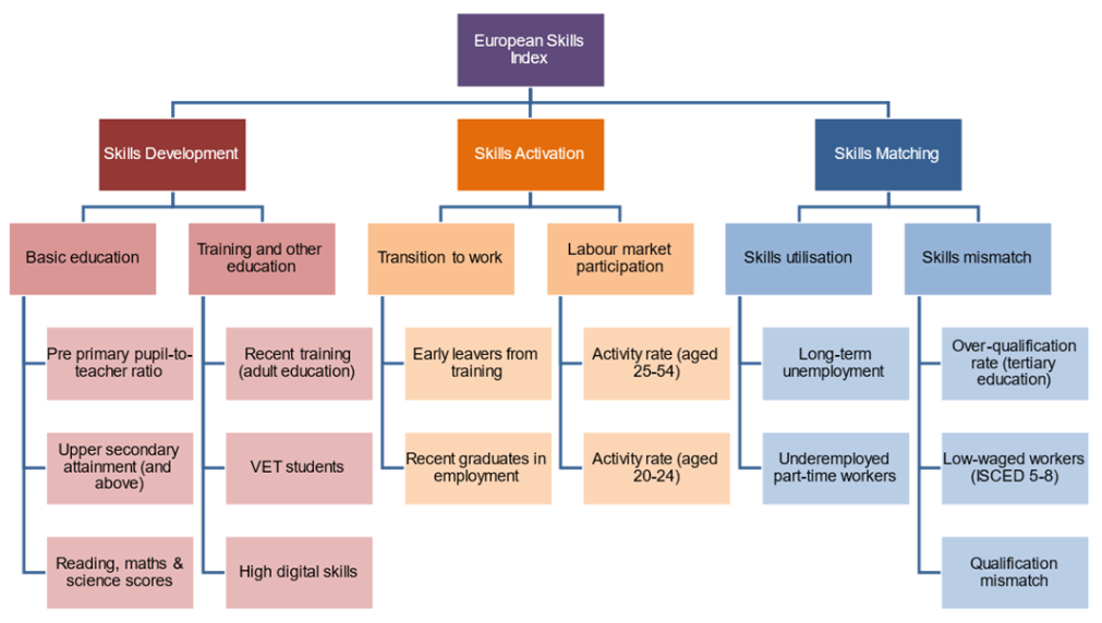
Rather than dreaming up a new composite indicator, we will recreate the European Skills Index, which is a composite indicator with 15 indicators measuring skills in European countries. Actually, we will miss out three of these indicators for reasons explained below, so this is only a partial recreation of the index.
Data collection
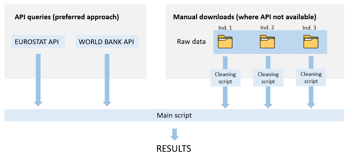
One way of collecting data is to download it from Eurostat in e.g. Excel or CSV, then merge together the different indicators. Then if we are building the CI in R, we would have to import it into R. etc. This approach will work but is slow if you need to update, and it is very easy to make mistakes. Also there is no record of exactly where you went to get your data.
A better way in many cases is to download the data directly into R via an “API”. R has many packages which provide easy interfaces to specific APIs - in our case, the eurostat package can be used to download Eurostat data directly into R. We will now use this to download our selected indicators.
Note that since this takes a minute or so, depending on the download speed, we will also save the raw data so that each time this document is generated, we don’t have to download again. This is effectively caching the data, but of course we always have the option to re-download the data if we suspect that indicators have been updated.
The following is how the data is downloaded. This code chunk will not be run except for (a) the first time we acquire the data, or (b) if we want to check for updates:
Notice that we reference Eurostat indicator codes (these can be found on the Eurostat website), and for each indicator we only download the relevant data using the filter options.
This list of indicators misses three indicators to properly recreate the ESI: namely PISA scores, low-waged workers and qualification mismatch. These three indicators are not directly downloadable from Eurostat. In practice, the raw data would be saved in three separate files (e.g. csv, Excel or similar), then a separate script would be written for each indicator, to clean and process it. It would then be gathered together with the other indicators here, the idea being to have a reproducible record of how we arrived at the final result, from the raw data. However, to keep things simple here we will simply omit these indicators in this example.
As mentioned, to avoid repeatedly downloading the same data, we will load a locally-saved version of the data:
l_data <- readRDS("raw_data.RDS")At this point we have all the data, but it needs tidying up: our data covers multiple years, has different columns and may not always include the same set of countries. Begin by converting the list into one big table with common columns:
# select relevant columns from each data set
l_data_filt <- lapply(names(l_data), function(iCode){
  X <- l_data[[iCode]]
  X <- X[c("geo", "time", "values")]
  X$iCode <- iCode
  X
})

# convert to table
df_data <- Reduce(rbind, l_data_filt)

# rename columns
names(df_data) <- c("uCode", "Time", "Value", "iCode")
Now we filter to EU27 countries:
# get EU27 country codes (use countrycode package, manually exclude UK)
countries <- countrycode::codelist[
  which((countrycode::codelist$eu28 == "EU") & (countrycode::codelist$eurostat != "UK")),
  c("country.name.en", "eurostat")
]
names(countries) <- c("uName", "uCode")

df_data <- df_data[df_data$uCode %in% countries$uCode, ]
At this point we have all of our data in a single long table. We have multiple years of data, so we want to know which years we have data for all indicators:
table(df_data[c("iCode", "Time")]) |>
  as.data.frame.matrix() |>
  DT::datatable(options = list(pageLength = 12))
This shows the counts of years against indicators, and shows that the latest year with all 27 countries having data for all indicators is 2019. So we use that in our example.
To note that COINr can deal with panel data easily, but for simplicity we will stick with a single year of data, so let’s filter to that.
df_data <- df_data[df_data$Time == 2019, ]
# see first few rows
head(df_data)
uCode Time Value iCode
25 BE 2019 NA PTRatio
34 BG 2019 12.1 PTRatio
43 CZ 2019 13.0 PTRatio
52 DK 2019 7.5 PTRatio
61 DE 2019 7.4 PTRatio
70 EE 2019 8.2 PTRatioNow we have a clean and focused data set. What remains is to format it for entry into COINr.
Formatting for COINr
To enter the data into COINr we need to build two tables:
- The indicator data (iData)
- The indicator metadata, including the index structure (iMeta)
These tables, the details of their construction and much other information, can be found in the COINr online documentation. When the tables are constructed, we will use COINr to build the composite indicator.
iData
The first data frame, iData specifies the value of each indicator, for each unit. It can also contain further attributes and metadata of units, for example groups, names, and denominating variables (variables which are used to adjust for size effects of indicators).
In our example this is fairly straightforward: we just pivot the table previously downloaded:
# pivot to wide
iData <- tidyr::pivot_wider(df_data, names_from = "iCode", values_from = "Value")

# remove time column
iData <- iData[names(iData) != "Time"]

# also add country names
iData <- merge(countries, iData)
Now our data set looks like this and is ready for entry into COINr:
DT::datatable(iData, rownames = F)iMeta
The iMeta data frame specifies everything about each column in iData, including whether it is an indicator, a group, or something else; its name, its units, and where it appears in the structure of the index. iMeta also requires entries for any aggregates which will be created by aggregating indicators.
This table requires some manual construction. We have to define indicator codes, names, directions, and the index structure. The structure of the iMeta table is a bit more complicated than the iData table, but it is explained thoroughly in the COINr documentation.
To be quick, we will just make the indicator names the same as codes for the moment. The following is the basic structure of the table which we will add to and edit:
iMeta <- data.frame(
  iCode = unique(df_data$iCode),
  iName = unique(df_data$iCode),
  Direction = 1,
  Level = 1,
  Weight = 1,
  Type = "Indicator"
)
Next we will edit the directions: some of our indicators have a negative directionality (associated with lower values of skills).
# indicators with negative directionality
neg_directions <- c("PTRatio" , "LeaveTrain", "LTUnemp", "UnderEmpPT", "OverQual")

# update iMeta
iMeta$Direction[iMeta$iCode %in% neg_directions] <- -1
Next we have to define the structure of the index. This is done by first assigning each indicator to its aggregation group using the “Parent” column, then adding additional rows to define the aggregates themselves (the pillars, etc, up to the index).
Defining the iMeta table may often be easier in Excel or similar, but here will do everything in R. First we assign the indicators to their groups in Level 2:
# assign level 2 groupings
iMeta$Parent <- c("BasicEd", "BasicEd",
                  "TrainEd", "TrainEd", "TrainEd",
                  "TransWork", "TransWork",
                  "ActRate", "ActRate",
                  "SkillUtil", "SkillUtil",
                  "SkillMisMa")
Now we must define level 2 itself:
iMeta_L2 <- data.frame(
  iCode = c("BasicEd", "TrainEd", "TransWork", "ActRate", "SkillUtil", "SkillMisMa"),
  iName = c("Basic Education", "Training and other education", "Transition to work",
            "Labour Market Participation", "Skills utilisation", "Skills mismatch"),
  Direction = 1,
  Level = 2,
  Weight = 1,
  Type = "Aggregate",
  Parent = c("SkillDev", "SkillDev", "SkillAct", "SkillAct", "SkillMatch", "SkillMatch")
)

# add to iMeta
iMeta <- rbind(iMeta, iMeta_L2)
Now define the final rows (level 3 and the index level 4):
iMeta_L34 <- data.frame(
  iCode = c("SkillDev", "SkillAct", "SkillMatch", "ESI"),
  iName = c("Skills development", "Skills activation", "Skills matching", "European Skills Index"),
  Direction = 1,
  Level = c(3,3,3,4),
  Weight = 1,
  Type = "Aggregate",
  Parent = c("ESI", "ESI", "ESI", NA)
)

# add to iMeta
iMeta <- rbind(iMeta, iMeta_L34)
The iMeta table is now complete. Let’s see what it looks like:
DT::datatable(iMeta, rownames = F)For the purposes of this example, we will also export both the indicator data and metadata to Excel to have a look at it.
openxlsx::write.xlsx(list(iData = iData, iMeta = iMeta), "ESI_COINr_input.xlsx")Initial analysis
We are now ready to actually use COINr. To use COINr we have to begin by building a “coin”, which is an object which contains all information about our composite indicator (data, structure, results, etc).
library(COINr)

ESI <- new_coin(iData, iMeta)
iData checked and OK.iMeta checked and OK.Written data set to .$Data$RawWe can check the contents of our coin at a glance:
ESI--------------
A coin with...
--------------
Input:
Units: 27 (AT, BE, BG, ...)
Indicators: 12 (Emp25_54, Emp20_24, PTRatio, ...)
Denominators: 0 ()
Groups: 0 (none)
Structure:
Level 1 : 12 indicators (Emp20_24, Emp25_54, EmpGrads, ...)
Level 2 : 6 groups (ActRate, TransWork, BasicEd, ...)
Level 3 : 3 groups (SkillAct, SkillDev, SkillMatch)
Level 4 : 1 groups (ESI)
Data sets:
Raw (27 units)We can also plot the index structure:
plot_framework(ESI)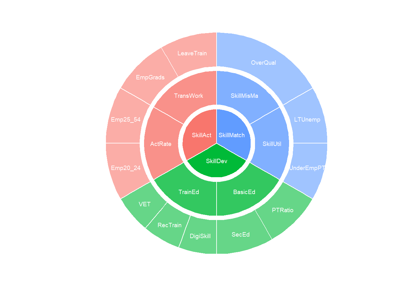
If we are working in HTML we can also use the iCOINr package for an interactive version:
library(iCOINr)
iplot_framework(ESI)
Another useful initial operation is to check indicator statistics:
get_stats(ESI, dset = "Raw") |>
  DT::datatable(rownames = F)
This can help us to flag initial problems. We may also wish to check correlations:
plot_corr(ESI, dset = "Raw", grouplev = 3, box_level = 2, use_directions = TRUE)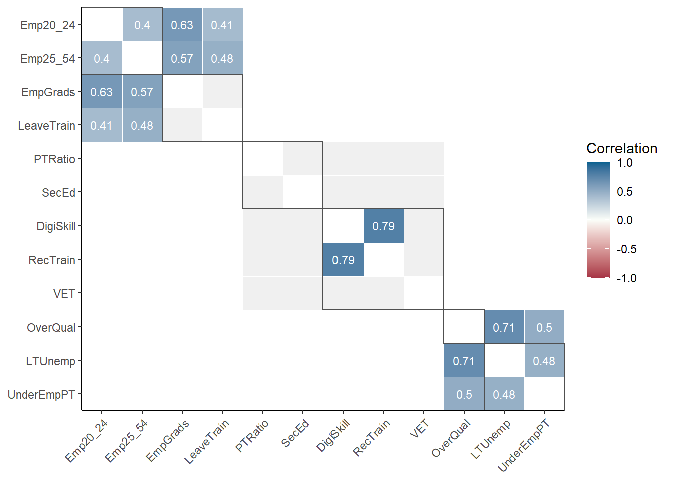
We can also plot the distributions of any indicators, including all indicators at once:
plot_dist(ESI, dset = "Raw", iCodes = "ESI", Level = 1)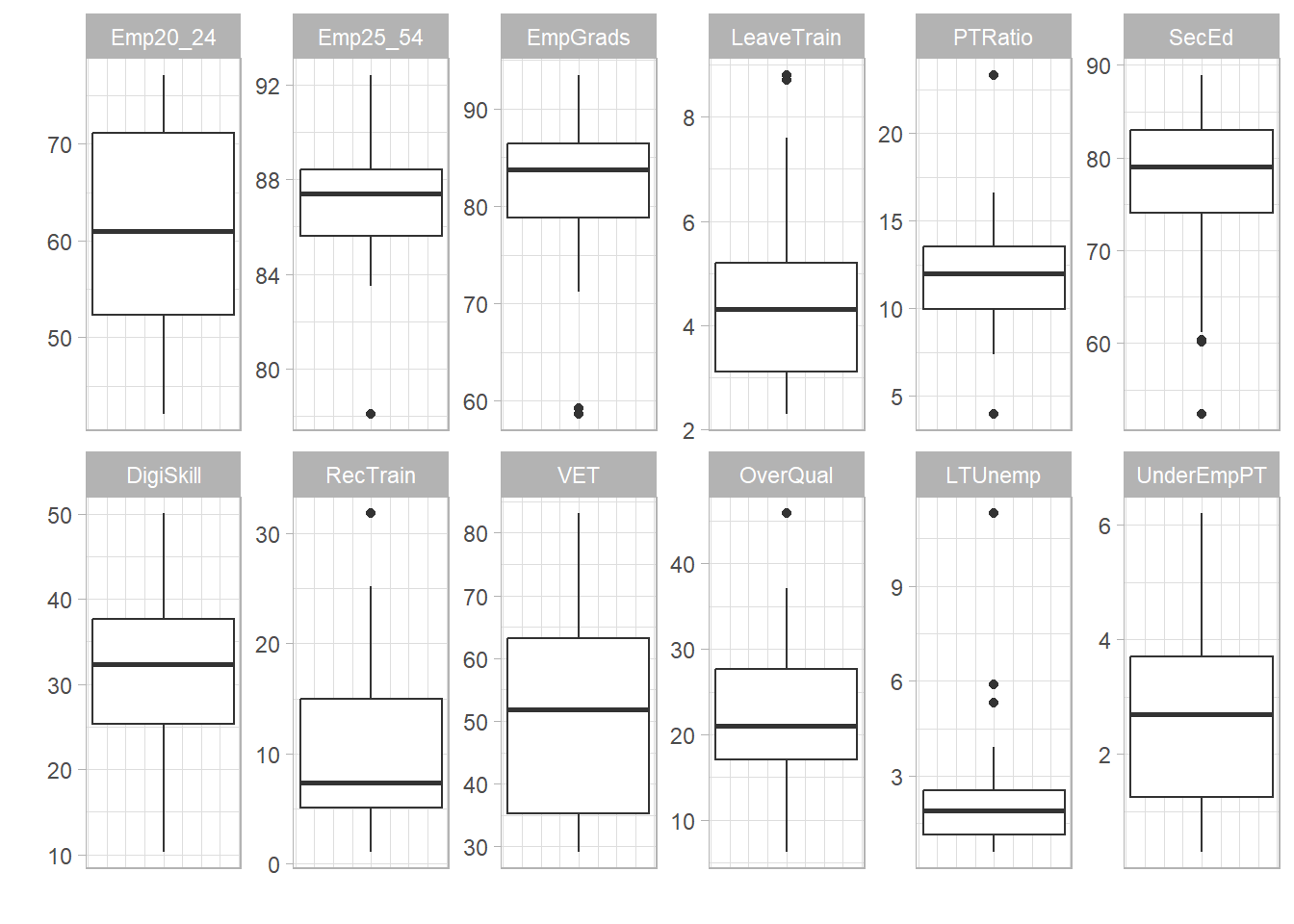
Further information on these steps can be found in the Statistical Analysis section of the online documentation.
Building the index
We will not follow the real ESI methodology here, but go for some very simple options in building the composite indicator.
First we will apply data treatment using a standard Winsorisation approach:
ESI <- qTreat(ESI, dset = "Raw", winmax = 5)Written data set to .$Data$TreatedLet us see what data treatment has been applied:
ESI$Analysis$Treated$Dets_Table |>
  signif_df() |>
  DT::datatable(rownames = F)
This table shows that only one data point was Winsorised, in the “LTUnemp” indicator. We may wish to visualise the difference between the treated and untreated indicator:
iCOINr::iplot_scatter(ESI, dsets = c("Raw", "Treated"), iCodes = "LTUnemp", Levels = 1)In COINr there are many options for data treatment, including changing the number of Winsorised points, the type of nonlinear transformation, and even building your own outlier treatment procedure using other packages. Details on data treatment are in the online documentation.
Next we can normalise the data:
ESI <- qNormalise(ESI, dset = "Treated")Written data set to .$Data$NormalisedBy default this uses the min-max method on the 0-100 interval. To confirm this we can plot the normalised data set as histograms:
plot_dist(ESI, dset = "Normalised", iCodes = "ESI", Level = 1, type = "Dot")Bin width defaults to 1/30 of the range of the data. Pick better value with
`binwidth`.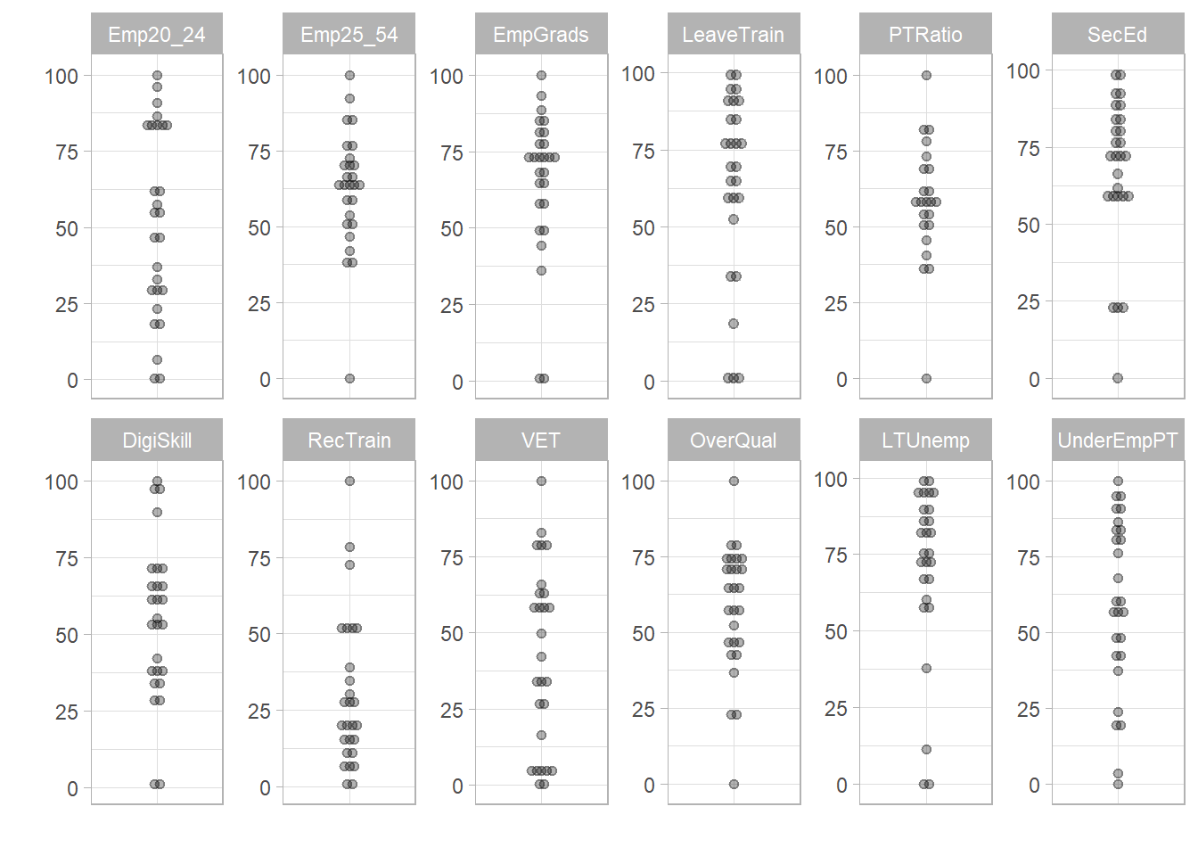
In COINr there are many alternative normalisation options, including:
- Z-scores
- Ranks
- Percentile ranks
- Borda scores
- Distance to target
- Distance to a reference unit
- Goalposts
- Using a custom normalisation method
Again, please see the documentation for full details.
Finally we aggregate the index using the good old arithmetic mean.
ESI <- Aggregate(ESI, dset = "Normalised", f_ag = "a_amean")Written data set to .$Data$AggregatedThe aggregation function will use the weights that were entered in the iMeta table at the beginning. You can however create new weight sets and store them in the coin, and also reweight using PCA or optimisation approaches. More on this is found in the relevant documentation chapter
Aggregation alternatives built into COINr are:
- Geometric mean (low compensation)
- Harmonic mean (even lower compensation)
- The Copeland method
- Use your own custom function
For the latter, this lets us use advanced aggregation methods such as DEA and others - some interesting approaches are available in the compind package - an example of using this with COINr is here.
We have now calculated our results, but they are still inside the coin. To view them easily we can call a helper function:
get_results(ESI, dset = "Aggregated", tab_type = "Full") |>
  DT::datatable(rownames = F)
Visualising results
There are many options for visualising the results. We begin with a bar chart:
plot_bar(ESI, dset = "Aggregated", iCode = "ESI", stack_children = TRUE)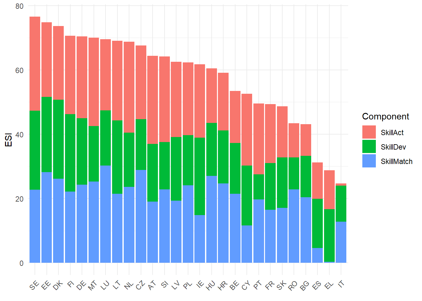
This can also be viewed using the iCOINr package:
iplot_bar(ESI, dset = "Aggregated", "ESI", orientation = "vertical", ulabs = "uName", stack_children = TRUE, ilabs = "iName")We may also wish to make a scatter plot, again this can be done in static or interactive mode:
iplot_scatter(ESI, dsets = c("Raw", "Aggregated"), iCodes = c("PTRatio", "ESI"), Levels = c(1, 4), axes_label = "iName", trendline = TRUE)Next we will plot our results on a map. This is outside of COINr but useful to know.
# first, acquire country shape files from Eurostat
SHP_0 <- eurostat::get_eurostat_geospatial(resolution = 10, nuts_level = 0, year = 2021)

# extract data from coin and join to the shape df
df_ESI <- get_data(ESI, dset = "Aggregated", iCodes = "ESI")
# merge data into shape df
SHP_0 <- base::merge(SHP_0, df_ESI, by.x = "CNTR_CODE", by.y = "uCode")

library(leaflet)

# Create a color palette for the map:
mypalette <- colorNumeric(palette = "Blues", domain = SHP_0$ESI, na.color = "transparent")

# now plot
leaflet(SHP_0) |>
  leaflet::addProviderTiles("CartoDB.Positron") |>
  leaflet::addPolygons(layerId = ~CNTR_CODE,
                       fillColor = ~mypalette(ESI),
                       weight = 2,
                       opacity = 1,
                       color = "white",
                       dashArray = "3",
                       fillOpacity = 0.7,
                       highlightOptions = leaflet::highlightOptions(
                         weight = 5,
                         color = "#666",
                         dashArray = "",
                         fillOpacity = 0.7,
                         bringToFront = TRUE)) |>
  leaflet::addLegend(pal = mypalette, values = ~ESI, opacity = 0.7, title = NULL,
                       position = "bottomright")
This map can be further customised and improved, but we won’t go any further here.
Recall that these results are not the same as the real ESI results because (a) we have omitted three indicators, and (b) we have followed a simplified methodology to keep this example simple.
Post-processing
Next we will run through a few post-processing/adjustment tasks.
Adjustments
Coins can easily be copied, modified and compared. To find out more about this, see the online documenation. Here, we will check what would happen if instead of using min-max normalisation we were to use percentile ranks.
# copy index
ESI_pr <- ESI

# modify - set normalisation method
ESI_pr$Log$qNormalise$f_n <- "n_prank"
ESI_pr$Log$qNormalise$f_n_para <- list(NULL)

# regen
ESI_pr <- Regen(ESI_pr)

# compare
compare_coins(ESI, ESI_pr, dset = "Aggregated", iCode = "ESI", also_get = "uName", sort_by = "coin.1") |>
  DT::datatable(rownames = FALSE)
We can see that there are differences: with the rank approach Estonia is the top performer.
Export
Most likely we will want to pass our results back outside R. COINr has a quick way to export the full coin contents to Excel.
# attach results table to coin first
ESI <- get_results(ESI, dset = "Aggregated", tab_type = "Full", dset_indicators = "Raw", out2 = "coin")

# export
export_to_excel(ESI, "ESI_results.xlsx")
Conclusions
This was a brief tour of some of the features of COIN. However, COINr can do many other things which we have not explored here:
- Global sensitivity analysis
- Effect of removing indicators
- Principal component analysis
- Imputation of missing data
- Time series analysis (handling and analysing panel data)
- Denomination
- Screening units based on missing data
- Reweighting e.g. using PCA, weight optimisation
… and many other things.
Overall we have demonstrated here how a composite indicator can be built from start to finish (excluding qualitative tasks like conceptual development, etc) in a fully reproducible way.